Linkers
Review of all the linkers implemented in ByoTrack. For more details, have a look at the documentation or implementation of each linker. ___________________________________________________
NearestNeighborLinker (Frame by frame linker using euclidean distance association)
KalmanLinker (Frame by frame linker that models motion with Kalman filters and use maximum likelihood association
KOFTLinker (Frame by frame linker that models motion using Optical Flow enhanced Kalman filters and maximum likelihood association)
IcyEMHTLinker (Wrapper around Icy EMHT algorithm that uses Kalman filters and multiple hypothesis association)
TrackMateLinker (Wrapper around u-track/TrackMate from Fiji. It uses Kalman filters and euclidean distance based association)
[1]:
import cv2
import numpy as np
import matplotlib as mpl
import matplotlib.pyplot as plt
import torch

import byotrack
import byotrack.example_data
import byotrack.visualize
Load a video
[2]:
# Open an example video
video = byotrack.example_data.hydra_neurons()[130:]  # Let's start at frame 130 where the animal is contracting

# Or provide a path to one of your video
#video = byotrack.Video("path/to/video.ext")

# Or load manually a video as a numpy array
# video = np.random.randn(50, 500, 500, 3)  # T, H, W, C
[3]:
TEST = True  # Set to False to analyze a whole video

if TEST:
    video = video[:50]  # Temporal slicing to analyze only the first 50 frames
[4]:
# A transform can be added to normalize and aggregate channels

transform_config = byotrack.VideoTransformConfig(aggregate=True, normalize=True, q_min=0.01, q_max=0.999, smooth_clip=1.0)
video.set_transform(transform_config)

# Show the min max value used to clip and normalize
print(video._normalizer.mini, video._normalizer.maxi)
[0.] [248.]
[5]:
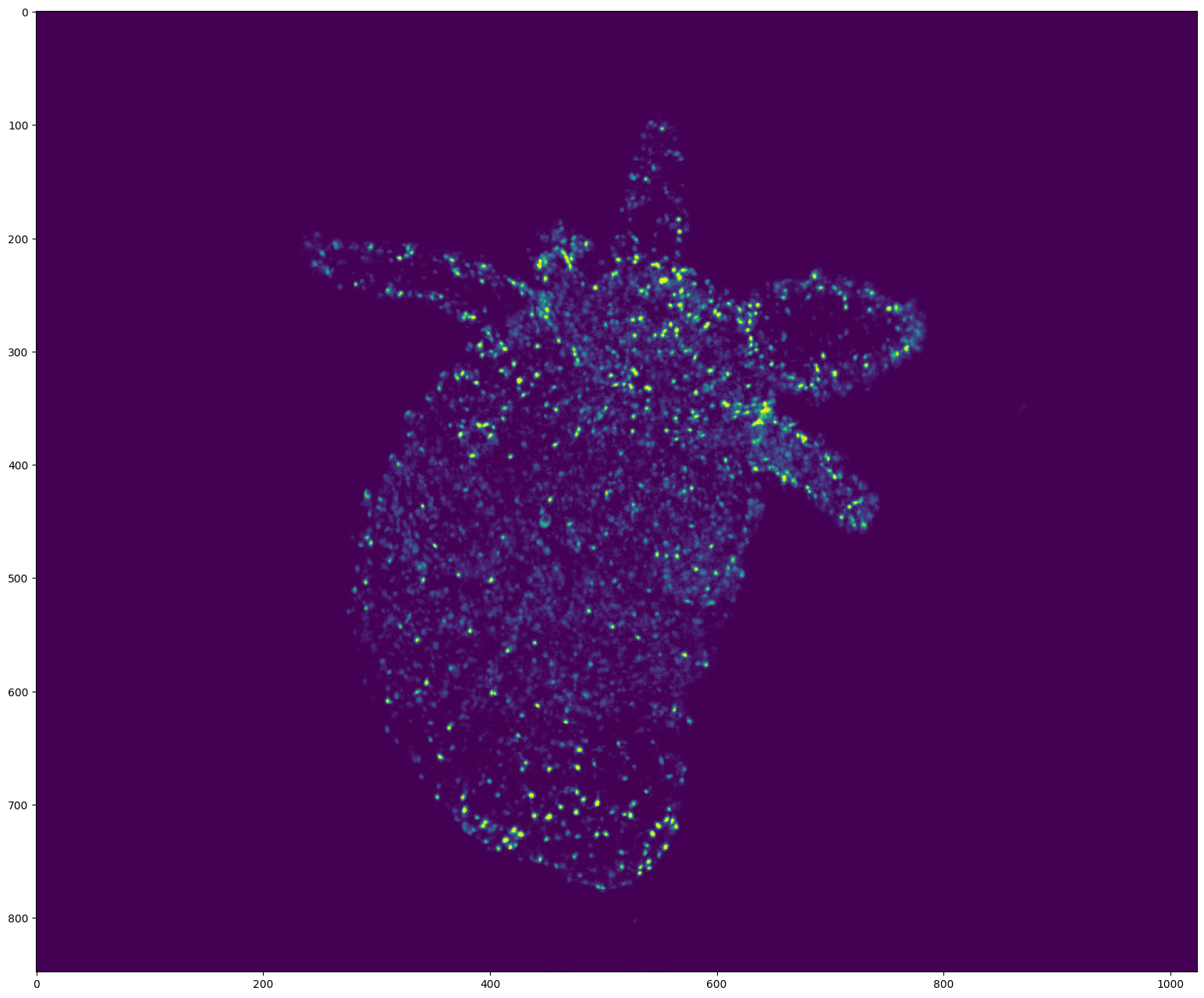
# Display the first frame

plt.figure(figsize=(24, 16), dpi=100)
plt.imshow(video[0])
plt.show()
[6]:
# Display the video with opencv
# Use w/x to move forward in time (or space to run/pause the video)
# Use v to switch on/off the display of the video

byotrack.visualize.InteractiveVisualizer(video).run()
Detections
The linker links detections through time. We use the WaveletDetector from byotrack as an example to produce the detections.
[7]:
# Create the detector object with its hyper parameters
from byotrack.implementation.detector.wavelet import WaveletDetector

detector = WaveletDetector(scale=1, k=3.0, min_area=5.0, batch_size=20, device=torch.device("cpu"))
[8]:
# Run the detection process on the current video

detections_sequence = detector.run(video)
[9]:
# Display the detections with opencv
# Use w/x to move forward in time (or space to run/pause the video)
# Use v to switch on/off the display of the video
# Use d to switch detection display mode (None, mask, segmentation)

byotrack.visualize.InteractiveVisualizer(video, detections_sequence).run()
NearestNeighborLinker
[10]:
from byotrack.implementation.linker.frame_by_frame.nearest_neighbor import NearestNeighborLinker, NearestNeighborParameters, AssociationMethod
[11]:
# See documentation about the Linker

NearestNeighborLinker?
[12]:
# See documentation about the Linker parameters

NearestNeighborParameters?
[13]:
# Create the linker
# We set only the main parameters
# You can look at the documentation to see the other ones

specs = NearestNeighborParameters(
    association_threshold=10.0,  # Most important one: Don't link if the euclidean distance is greater than 10 pixels
    n_valid=3,  # Validate a track after three consecutive detections
    n_gap=3,  # At most 3 consecutive missed detections
    association_method="opt_smooth"  # See AssociationMethod?, you can use greedy which is faster but usually less performant
)

linker = NearestNeighborLinker(specs)
[14]:
# Run the linker

tracks = linker.run(video, detections_sequence)
[15]:
# Display the tracks with opencv
# Use w/x to move forward in time (or space to run/pause the video)
# Use v (resp. t) to switch on/off the display of video (resp. tracks)
# Use d to switch detection display mode (None, mask, segmentation)

byotrack.visualize.InteractiveVisualizer(video, detections_sequence, tracks).run()
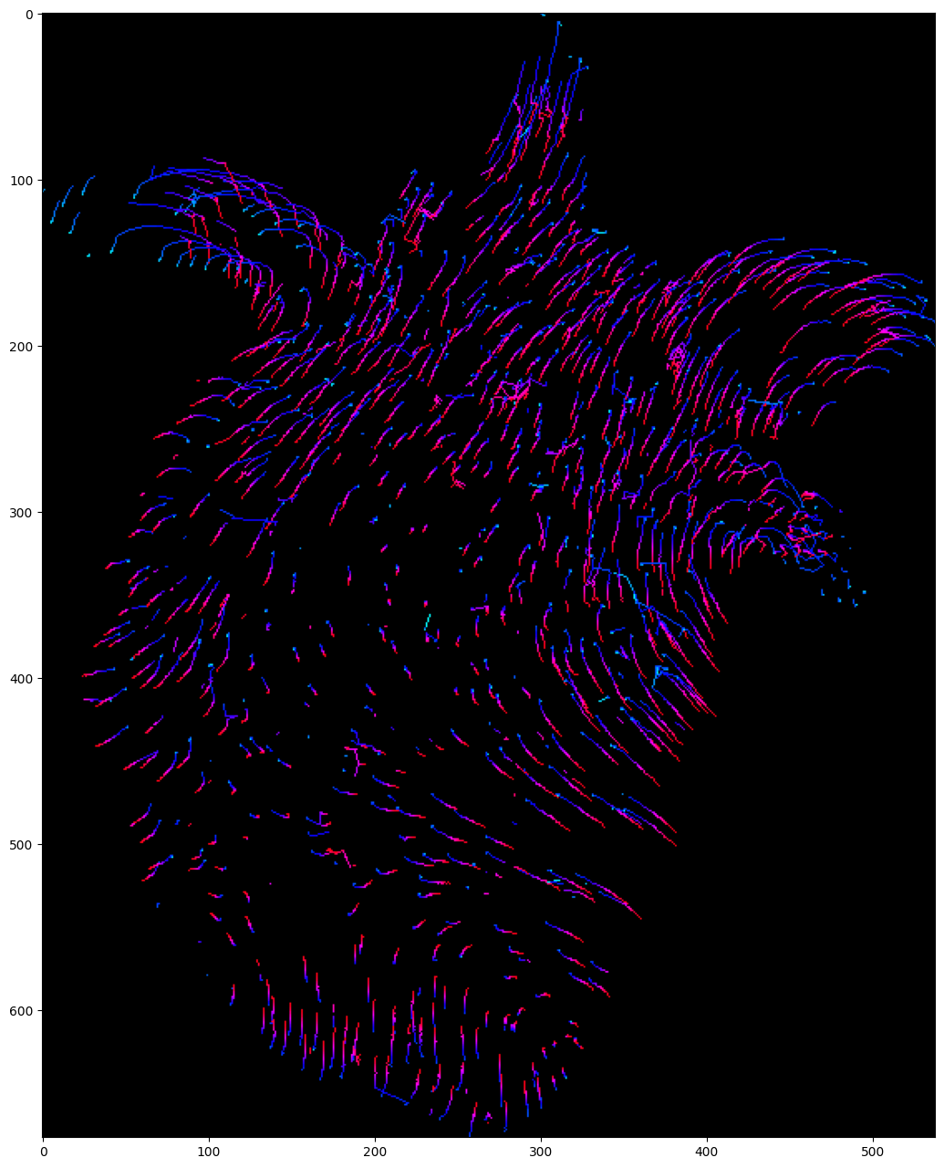
[16]:
# Project tracks onto a single image and color by time

# Create a list of colors for each time frame
# From cyan (start of the video) to red (end of the video)

hsv = mpl.colormaps["hsv"]
colors = [tuple(int(c * 255) for c in hsv(0.5 + 0.5 * k / (len(detections_sequence) - 1))[:3]) for k in range(len(detections_sequence))]

visu = byotrack.visualize.temporal_projection(
    byotrack.Track.tensorize(tracks),
    colors=colors,
    background=None,
    color_by_time=True
)

plt.figure(figsize=(24, 16))
plt.imshow(visu)
plt.show()

KalmanLinker
[17]:
from byotrack.implementation.linker.frame_by_frame.kalman_linker import KalmanLinker, KalmanLinkerParameters, Cost
[18]:
# See documentation about the Linker

KalmanLinker?
[19]:
# See documentation about the Linker parameters

KalmanLinkerParameters?
[20]:
# Create the linker
# We set only the main parameters.
# You can look at the documentation to see the other ones.

specs = KalmanLinkerParameters(
    association_threshold=1e-3,  # Most important parameter: don't link if the association likelihood is smaller than 1e-4.
    detection_std=3.0,  # Detections location are precise up to 3.0 pixels
    process_std=3.0,  # Kalman filter predictions are precise up to 3.0 pixels
    kalman_order=1,  # Order of the kalman filter
    cost="likelihood",  # See Cost? to see which other cost are available, by default it uses Euclidean distance (And association threshod should be express in pixels)
)

linker = KalmanLinker(specs)
[21]:
# Run the linker

tracks = linker.run(video, detections_sequence)
[22]:
# Display the tracks with opencv
# Use w/x to move forward in time (or space to run/pause the video)
# Use v (resp. t) to switch on/off the display of video (resp. tracks)
# Use d to switch detection display mode (None, mask, segmentation)

byotrack.visualize.InteractiveVisualizer(video, detections_sequence, tracks).run()
[23]:
# Project tracks onto a single image and color by time

# Create a list of colors for each time frame
# From cyan (start of the video) to red (end of the video)

hsv = mpl.colormaps["hsv"]
colors = [tuple(int(c * 255) for c in hsv(0.5 + 0.5 * k / (len(detections_sequence) - 1))[:3]) for k in range(len(detections_sequence))]

visu = byotrack.visualize.temporal_projection(
    byotrack.Track.tensorize(tracks),
    colors=colors,
    background=None,
    color_by_time=True
)

plt.figure(figsize=(24, 16))
plt.imshow(visu)
plt.show()

KOFTLinker
[24]:
from byotrack.implementation.linker.frame_by_frame.koft import KOFTLinker, KOFTLinkerParameters
[25]:
# See documentation about the Linker

KOFTLinker?
[26]:
# See documentation about the Linker parameters

KOFTLinkerParameters?
[27]:
# Koft requires optical flow (NOTE: that optical flow can also be efficiently be used with the two previous linker)

# You could use any optical flow algorithm, but ByoTrack already supports OpenCV and Skimage implementations.
# Let's use Farneback from OpenCV (no extra dependencies)

import cv2
from byotrack.implementation.optical_flow.opencv import OpenCVOpticalFlow

optflow = OpenCVOpticalFlow(cv2.FarnebackOpticalFlow_create(winSize=20), downscale=4)
[28]:
# Before linking, let's check visually that the optical flow algorithm works
# We sample a grid of points that are moved by the flow computed.
# The computed flows are good if the points roughly follows the video motion

# Use w/x to move forward in time (or space to run/pause the video)
# Use g to reset the grid of points

byotrack.visualize.InteractiveFlowVisualizer(video, optflow).run()
[29]:
# Create the linker
# We set only the main parameters.
# You can look at the documentation to see the other ones.

specs = KOFTLinkerParameters(
    association_threshold=2e-3,  # Most important parameter: don't link if the association likelihood is smaller than 1e-3.
    detection_std=3.0,  # Detections location are precise up to 3.0 pixels
    process_std=1.5,  # Kalman filter predictions are precise up to 3.0 pixels
    flow_std=1.0,  # Optical flow predictions are precise up to 1.0 pixels/frame
    kalman_order=1,  # Order of the kalman filter
    n_gap=5,  # Allow to link after 5 consecutive missed detections
    cost="likelihood",  # See Cost? to see which other cost are available, by default it uses Euclidean distance (And association threshod should be express in pixels)
)

linker = KOFTLinker(specs, optflow)
[30]:
# Run the linker

tracks = linker.run(video, detections_sequence)
[31]:
# Display the tracks with opencv
# Use w/x to move forward in time (or space to run/pause the video)
# Use v (resp. t) to switch on/off the display of video (resp. tracks)
# Use d to switch detection display mode (None, mask, segmentation)

byotrack.visualize.InteractiveVisualizer(video, detections_sequence, tracks).run()
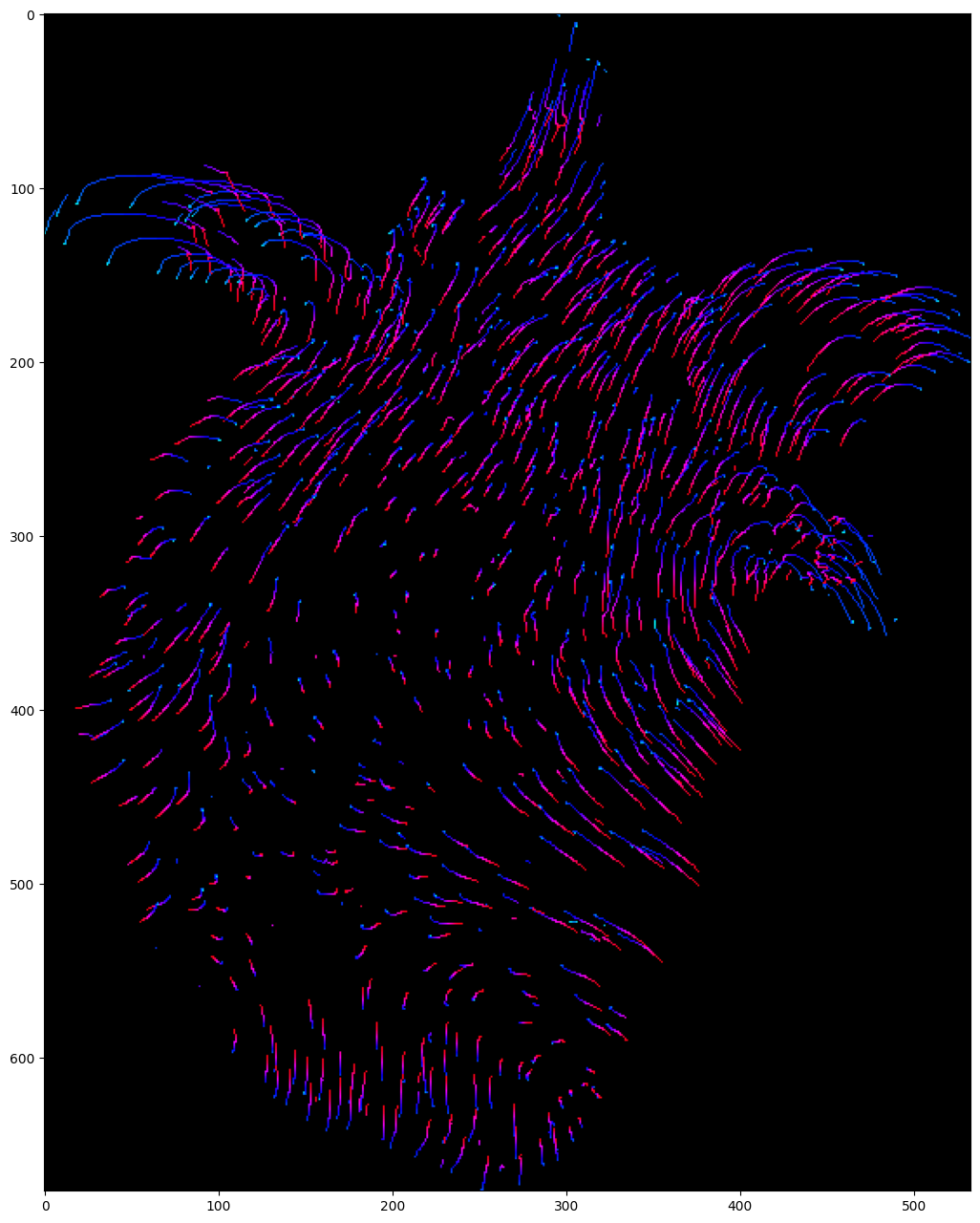
[32]:
# Project tracks onto a single image and color by time

# Create a list of colors for each time frame
# From cyan (start of the video) to red (end of the video)

hsv = mpl.colormaps["hsv"]
colors = [tuple(int(c * 255) for c in hsv(0.5 + 0.5 * k / (len(detections_sequence) - 1))[:3]) for k in range(len(detections_sequence))]

visu = byotrack.visualize.temporal_projection(
    byotrack.Track.tensorize(tracks),
    colors=colors,
    background=None,
    color_by_time=True
)

plt.figure(figsize=(24, 16))
plt.imshow(visu)
plt.show()
EMHT (Icy)
Icy software must be installed
[33]:
from byotrack.implementation.linker.icy_emht import IcyEMHTLinker, Motion, EMHTParameters
[34]:
# See documentation about the Linker

IcyEMHTLinker?
[35]:
# See documentation about the Linker parameters

EMHTParameters?
[36]:
# Create the linker object with icy path
# This Linker requires to install Icy software first

icy_path = "path/to/icy/icy.jar"
motion = Motion.MULTI  # Can also be DIRECTED or MULTI (both)

if True:  # Set full specs with EMHTParameters
    # You can choose to set manually the parameters. See EMHTParameters
    # the more important ones are:
    # - gate_factor: How greedy the linking is. (Default to 4.0) more or less equivalent to the association_threshold
    #       of KalmanLinker with a Mahalanobis Cost.
    # - motion: Motion model to consider: Can be BROWNIAN, DIRECTED or MULTI. (Default is BROWNIAN)
    #       Brownian <=> kalman_order = 0, Directed <=> kalman_order = 1 (MULTI uses both)
    # - tree_depth: MHT tree depth. Higher values are usually more performant, but much more expensive
    #             If the tracking is too slow or too ram intensive, you may reduce this value. (Default 4)
    parameters = EMHTParameters(gate_factor=4.0, motion=motion, tree_depth=2)
    linker = IcyEMHTLinker(icy_path, parameters)
else:  # Do not provide specs, parameters will be estimated by Icy (We do not advise this solution)
    linker = IcyEMHTLinker(icy_path)
    linker.motion = motion  # Set motion afterwards if no parameters are provided
[37]:
# Run the linker

tracks = linker.run(video, detections_sequence)
Calling Icy with: java -jar icy.jar -hl -x plugins.adufour.protocols.Protocols protocol="/home/rreme/workspace/pasteur/byotrack/byotrack/implementation/linker/icy_emht/emht_protocol_with_full_specs.xml" rois="/home/rreme/workspace/pasteur/byotrack/docs/source/run_examples/_tmp_rois.xml" parameters="/home/rreme/workspace/pasteur/byotrack/docs/source/run_examples/_tmp_parameters.xml" tracks="/home/rreme/workspace/pasteur/byotrack/docs/source/run_examples/_tmp_tracks.xml"
[DEBUG] 2024-07-04 15:25:22 - Initializing...
JarResources.loadJar(/home/rreme/workspace/pasteur/icy-app-v3/plugins/nchenouard/particletracking/sequenceGenerator/._tracking-benchmark-generator-2.0.0.jar) error:
java.util.zip.ZipException: zip END header not found
[INFO] 2024-07-04 15:25:22 - Java(TM) SE Runtime Environment 21.0.1+12-LTS-29 (64 bit)
[INFO] 2024-07-04 15:25:22 - Running on Linux 5.15.0-107-generic (amd64)
[INFO] 2024-07-04 15:25:22 - System total memory: 32.6 GB
[INFO] 2024-07-04 15:25:22 - System available memory: 5.7 GB
[INFO] 2024-07-04 15:25:22 - Max Java memory: 8.2 GB
[INFO] 2024-07-04 15:25:22 - Headless mode.
[INFO] 2024-07-04 15:25:22 - Icy v3.0.0a started.
[DEBUG] 2024-07-04 15:25:23 - Magic name is Spot Tracking
[DEBUG] 2024-07-04 15:25:23 - Magic icon is /plugins/nchenouard/particletracking/simplifiedMHT/detectionIcon.png
[DEBUG] 2024-07-04 15:25:23 - Magic name is EzPlug tutorial
[DEBUG] 2024-07-04 15:25:23 - Magic icon is /plugins/adufour/ezplug/ezplug.png
Loading workflow...
Error(s) while loading protocol:
Variable 'useLPSolver' not found in block 'Spot tracking do tracking'. It may have been removed or renamed.
--
Converted from 31443 ROI(s)
Non binaryaction at frame 3
Non binaryaction at frame 9
Non binaryaction at frame 46
Track extraction at frame 49
[INFO] 2024-07-04 15:25:38 - Exiting...
[INFO] 2024-07-04 15:25:38 - Done.
[38]:
# Display the tracks with opencv
# Use w/x to move forward in time (or space to run/pause the video)
# Use v (resp. t) to switch on/off the display of video (resp. tracks)
# Use d to switch detection display mode (None, mask, segmentation)

byotrack.visualize.InteractiveVisualizer(video, detections_sequence, tracks).run()
[39]:
# Project tracks onto a single image and color by time

# Create a list of colors for each time frame
# From cyan (start of the video) to red (end of the video)

hsv = mpl.colormaps["hsv"]
colors = [tuple(int(c * 255) for c in hsv(0.5 + 0.5 * k / (len(detections_sequence) - 1))[:3]) for k in range(len(detections_sequence))]

visu = byotrack.visualize.temporal_projection(
    byotrack.Track.tensorize(tracks),
    colors=colors,
    background=None,
    color_by_time=True
)

plt.figure(figsize=(24, 16))
plt.imshow(visu)
plt.show()

TrackMate (Fiji)
ImageJ/Fiji software must be installed
[40]:
from byotrack.implementation.linker.trackmate import TrackMateLinker, TrackMateParameters
[41]:
# See documentation about the Linker

TrackMateLinker?
[42]:
# See documentation about the Linker parameters

TrackMateParameters?
[43]:
# Create the linker object with fiji path
# This Linker requires to install Fiji software first
# We set only the main parameters.
# You can look at the documentation to see the other ones.

fiji_path = "path/to/Fiji.app/ImageJ-os"

specs = TrackMateParameters(
    linking_max_distance=10.0,  # Max linking euclidean distance (pixels) between consecutive spots
    max_frame_gap=4,  # Max diff in frames to allow gap closing. Here it allows 3 consecutives missed detections
    gap_closing_max_distance=15.0,  # Max gap closing euclidean distance (pixels).
    kalman_search_radius=10.0  # When set, it enables Kalman filters, and replace the linking_max_distance (except for the first two spots association)
)


linker = TrackMateLinker(fiji_path, specs)
[44]:
# Run the linker

tracks = linker.run(video, detections_sequence)
Calling Fiji with: ./ImageJ-linux64 --ij2 --headless --console --run "/home/rreme/workspace/pasteur/byotrack/byotrack/implementation/linker/trackmate/_trackmate.py" "detections='/home/rreme/workspace/pasteur/byotrack/docs/source/run_examples/_tmp_detections.tif',parameters='/home/rreme/workspace/pasteur/byotrack/docs/source/run_examples/_tmp_parameters.json',tracks='/home/rreme/workspace/pasteur/byotrack/docs/source/run_examples/_tmp_tracks.xml'"
OpenJDK 64-Bit Server VM warning: ignoring option PermSize=128m; support was removed in 8.0
OpenJDK 64-Bit Server VM warning: Using incremental CMS is deprecated and will likely be removed in a future release
Hello from ImageJ/Fiji
('Loading detections from', u'/home/rreme/workspace/pasteur/byotrack/docs/source/run_examples/_tmp_detections.tif')
Settings:
{u'MAX_FRAME_GAP': 4, u'ALTERNATIVE_LINKING_COST_FACTOR': 1.05, u'KALMAN_SEARCH_RADIUS': 10.0, u'LINKING_FEATURE_PENALTIES': {}, u'LINKING_MAX_DISTANCE': 10.0, u'GAP_CLOSING_MAX_DISTANCE': 15.0, u'MERGING_FEATURE_PENALTIES': {}, u'SPLITTING_MAX_DISTANCE': 15.0, u'BLOCKING_VALUE': inf, u'ALLOW_GAP_CLOSING': True, u'ALLOW_TRACK_SPLITTING': False, u'ALLOW_TRACK_MERGING': False, u'MERGING_MAX_DISTANCE': 15.0, u'SPLITTING_FEATURE_PENALTIES': {}, u'CUTOFF_PERCENTILE': 0.9, u'GAP_CLOSING_FEATURE_PENALTIES': {}}
Starting detection process using 16 threads.
Detection processes 16 frames simultaneously and allocates 1 thread per frame.
Detection...
Found 31443 spots.

Starting initial filtering process.
Computing spot features over 16 frames simultaneously and allocating 1 thread per frame.
Calculating 31443 spots features...

Computation done in 2 ms.
Starting spot filtering process.
Starting tracking process.
Creating the segment linking cost matrix...
Creating the main cost matrix...
Completing the cost matrix...
Solving the cost matrix...

Creating links...

Computing edge features:
Computation done in 0 ms.
Computing track features:
Computation done in 5 ms.
Starting track filtering process.
[45]:
# Display the tracks with opencv
# Use w/x to move forward in time (or space to run/pause the video)
# Use v (resp. t) to switch on/off the display of video (resp. tracks)
# Use d to switch detection display mode (None, mask, segmentation)

byotrack.visualize.InteractiveVisualizer(video, detections_sequence, tracks).run()
[46]:
# Project tracks onto a single image and color by time

# Create a list of colors for each time frame
# From cyan (start of the video) to red (end of the video)

hsv = mpl.colormaps["hsv"]
colors = [tuple(int(c * 255) for c in hsv(0.5 + 0.5 * k / (len(detections_sequence) - 1))[:3]) for k in range(len(detections_sequence))]

visu = byotrack.visualize.temporal_projection(
    byotrack.Track.tensorize(tracks),
    colors=colors,
    background=None,
    color_by_time=True
)

plt.figure(figsize=(24, 16))
plt.imshow(visu)
plt.show()