ByoTrack fundamental features
[1]:
import cv2
import matplotlib as mpl
import matplotlib.pyplot as plt
import numpy as np
import torch

import byotrack
import byotrack.example_data
import byotrack.napari  # For Napari visualization [REQUIRES NAPARI]
import byotrack.visualize
Loading a video
[2]:
# Open an example video
video = byotrack.example_data.hydra_neurons()[130:]  # Let's start at frame 130 where the animal is contracting

# Or provide a path to one of your video
# video = byotrack.Video("path/to/video.ext")

# Or load manually a video as a numpy array
# video = byotrack.Video(np.random.randn(50, 500, 500, 3))  # T, H, W, C
[3]:
TEST = True  # Set to False to analyze a whole video

if TEST:
    video = video[:50]  # Temporal slicing to analyze only the first 50 frames
[4]:
# Preprocess the video (normalization & channel aggregation)

print(video.shape, video.dtype)

video.add_preprocessor(byotrack.video.ChannelProjection("mean"))
video = video.normalize(q_min=0.01, q_max=0.999, smooth_clip=1.0)

print(video.shape, video.dtype)
(50, 848, 1024, 3) uint8
(50, 848, 1024, 1) float32
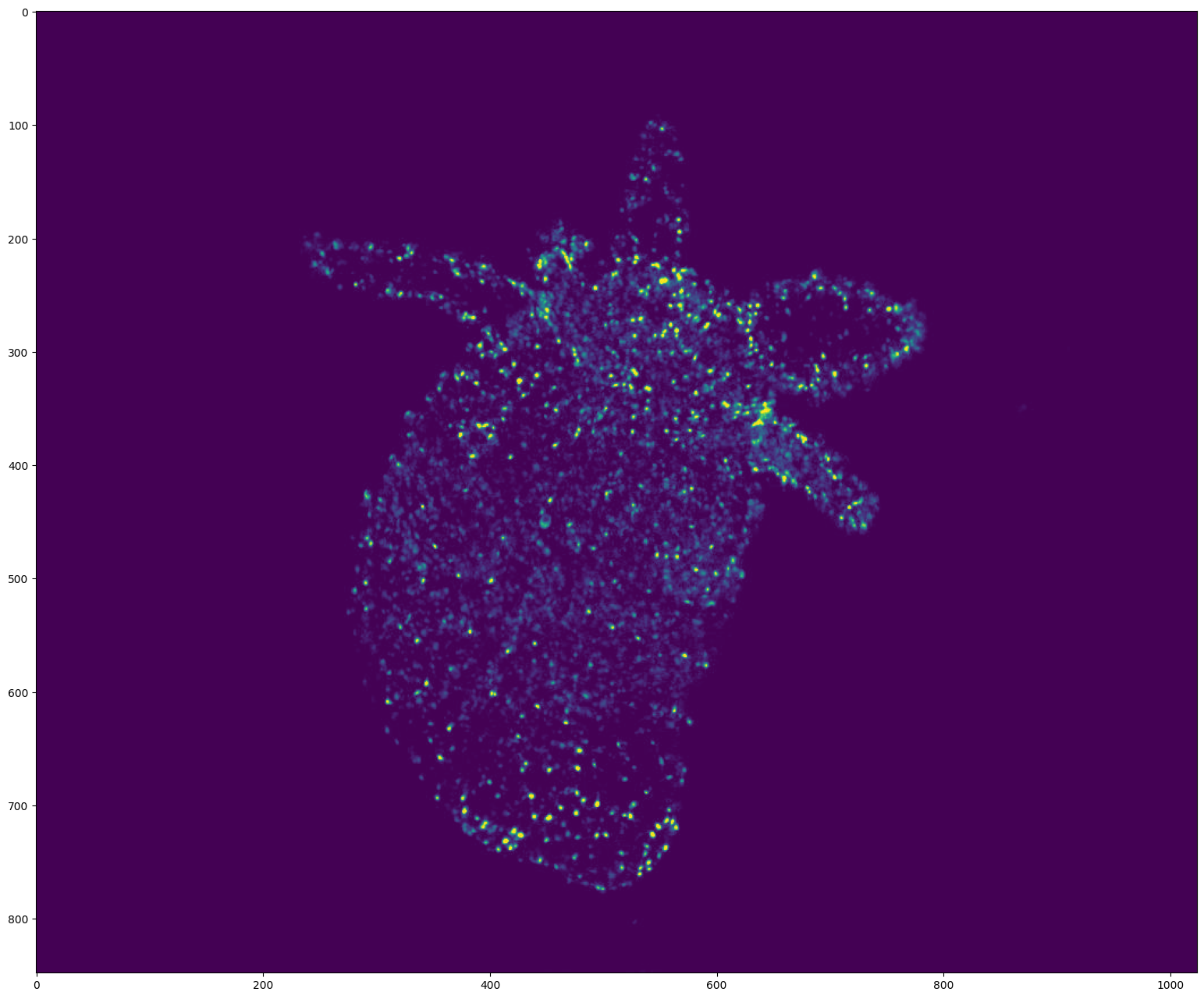
[5]:
# Display the first frame

frame = video[0]
if video.ndim == 5:  # (T, D, H, W, C) (3D video)
    frame = frame[frame.shape[0] // 2]  # Show the frame in the middle of the stack

plt.figure(figsize=(24, 16), dpi=100)
plt.imshow(frame)
plt.show()
[6]:
# Display the video with Napari

viewer = byotrack.napari.visualize(video)
Detections on a video: Example of WaveletDetector
[7]:
# Create the detector object with its hyper parameters
from byotrack.implementation.detector.wavelet import WaveletDetector

detector = WaveletDetector(scale=1, k=2.5, min_area=5, batch_size=20, device=torch.device("cpu"))
[8]:
# Run the detection process on the current video

detections_sequence = detector.run(video)
[9]:
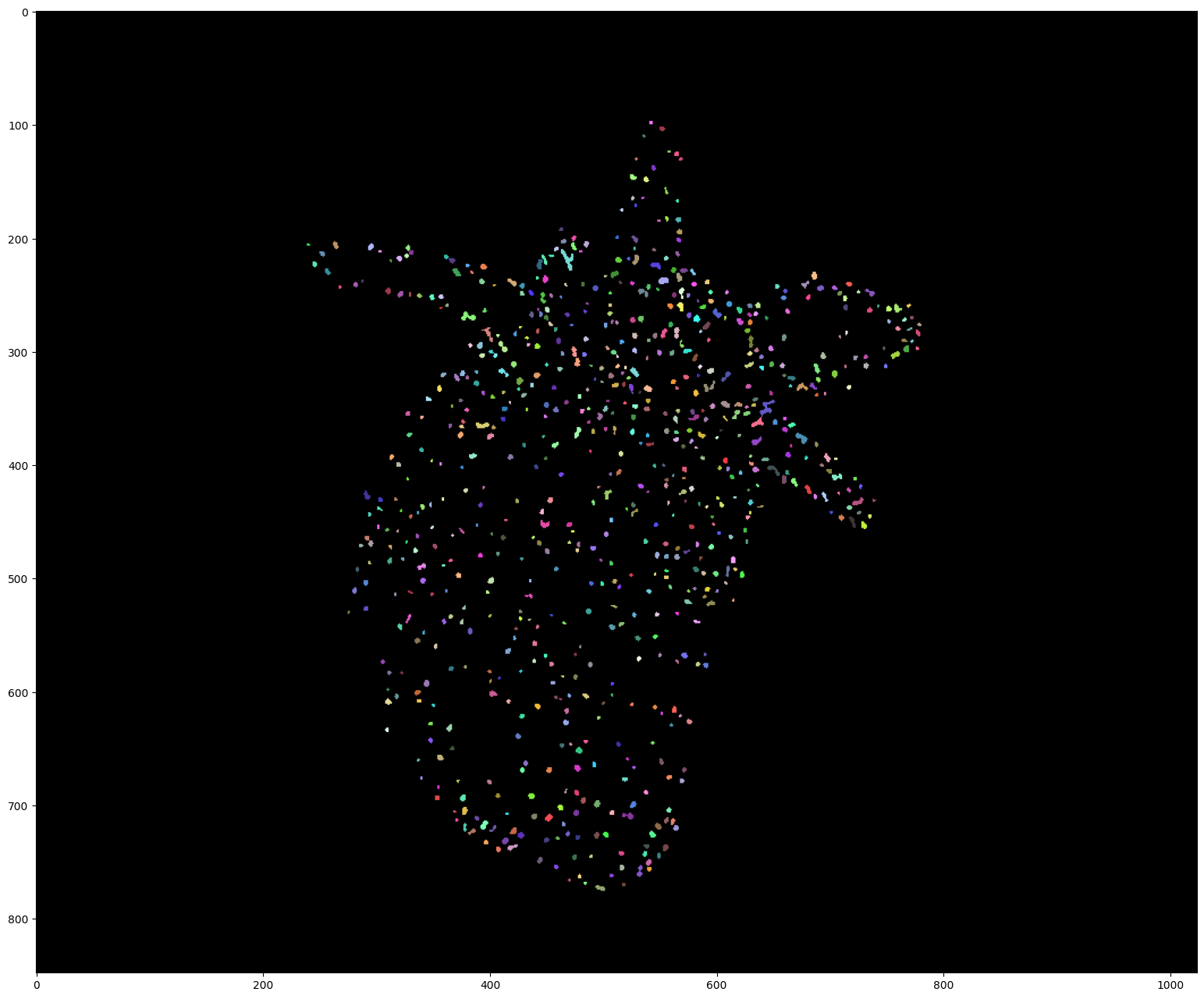
# Display the first detections

segmentation = detections_sequence[0].segmentation

if detections_sequence[0].dim == 3:  # 3D
    segmentation = segmentation[segmentation.shape[0] // 2]  # Show the segmentation in the middle of the stack

np.random.seed(0)
colors = np.random.randint(50, 255, (detections_sequence[0].length * 2, 3))
colors[0] = 0

plt.figure(figsize=(24, 16), dpi=100)
plt.imshow(colors[segmentation])
plt.show()
[10]:
# Display the video & detections with Napari

viewer = byotrack.napari.viewer.visualize(video, detections_sequence)
Link detections: Example of KOFTLinker (Kalman and Optical Flow Tracking)
[11]:
# KOFT requires Optical Flow. We give here the example of Farneback from Open-CV.

from byotrack.implementation.optical_flow.opencv import OpenCVOpticalFlow

# Prepare the optical flow algorithm
optflow = OpenCVOpticalFlow(cv2.FarnebackOpticalFlow_create(winSize=20), downscale=4)
[12]:
# Before linking, let's check visually that the optical flow algorithm works
# We sample a grid of points that are moved by the flow computed.
# The computed flows are good if the grid follows the video motion

# Use "g" to reset the grid of points

viewer = byotrack.napari.visualize_flow_deformation(video, optflow)
[13]:
from byotrack.implementation.linker.frame_by_frame.koft import KOFTLinker, KOFTLinkerParameters

# Create the linker
# Look at the documentation (KOFTLinkerParameters?) to see what parameters are available and their full descriptions

specs = KOFTLinkerParameters(
    association_threshold=1e-3,  # Most important parameter: don't link if the association likelihood is smaller than 1e-3.
    # Higher values will increase fragmentation of the trajectories. Lower values will reduce fragmentation but may increase identity switch.
    # Typical values are in [1e-5, 1e-2]
    detection_std=2.0,  # Detection precision (~ /3 of spot size)
    process_std=1.5,  # Motion prediction precision (~ /3 of unmodeled displacement)
    flow_std=1.0,  # Optical flow precision (Estimated around 1.0 pixels/frame)
    kalman_order=1,  # Order of the kalman filter (0: Brownian, 1: Directed, 2: Accelerated, ...)
    n_gap=5,  # Allow to link after 7 consecutive missed detections
    cost="likelihood",  # See koft.Cost? to see which other cost are available. Euclidean is usually less performant, but allows to express association_threshold in pixels.
    track_building="detection",  # Use detection position to build tracks. Note that you should rather use "smoothed" to remove NaNs and improve localization.
)

linker = KOFTLinker(specs, optflow)
[14]:
# Run the linker given a video and detections

tracks = linker.run(video, detections_sequence)
[15]:
# Visualize track lifetime

# Each track is in white when it alive. (Track on x-axis, time on y-axis)

byotrack.visualize.display_lifetime(tracks)

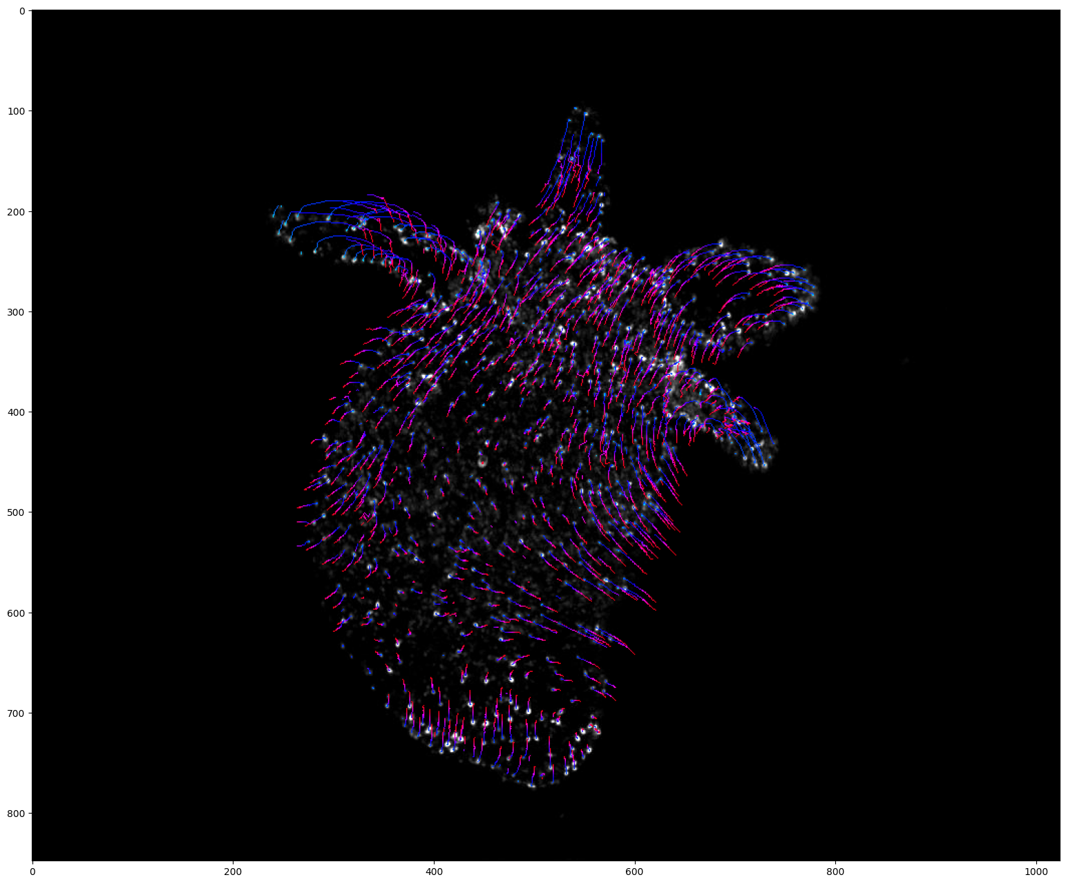
[16]:
# Project tracks onto a single image and color by time (Only works with 2D videos)

# Create a list of colors for each time frame
# From cyan (start of the video) to red (end of the video)

hsv = mpl.colormaps["hsv"]
colors = [
    tuple(int(c * 255) for c in hsv(0.5 + 0.5 * k / (len(detections_sequence) - 1))[:3])
    for k in range(len(detections_sequence))
]

visu = byotrack.visualize.temporal_projection(
    byotrack.Track.tensorize(tracks), colors=colors, background=video[0], color_by_time=True
)

plt.figure(figsize=(24, 16))
plt.imshow(visu)
plt.show()
[17]:
# Display the video, detections and tracks with Napari

viewer = byotrack.napari.visualize(video, detections_sequence, tracks)
Tracks refinement: Example of RTSSmoother, followed by EMC2 Stitcher
[18]:
from byotrack.implementation.refiner.interpolater import ForwardBackwardInterpolater
from byotrack.implementation.refiner.smoother import RTSSmoother
from byotrack.implementation.refiner.stitching import EMC2Stitcher
[19]:
# Smooth track positions using the optimal RTS smoothing method.
# This will improve position estimation if tracks are not smoothed yet.

smoother = RTSSmoother(detection_std=2.0, process_std=3.0, kalman_order=1)
tracks = smoother.run(video, tracks)
[20]:
# Visualize track lifetime

byotrack.visualize.display_lifetime(tracks)

[21]:
# Stitch tracks together in order to produce coherent track on all the video

stitcher = EMC2Stitcher(eta=5.0)  # Don't link tracks if they are too far (EMC dist > 5 (pixels))
tracks = stitcher.run(video, tracks)
Merging 1022 tracks into 964 resulting tracks
[22]:
# Visualize track lifetime

byotrack.visualize.display_lifetime(tracks)

[23]:
# After EMC2 stitching, NaN values can be inside merged tracks.
# It can be filled with interpolation between known positions

method = "tps"  # tps / constant / flow (You need to provided a valid byotrack.OpticalFlow then)
full = False  # Extrapolate position of the tracks on the all frame range and not just for the track lifespan

interpolater = ForwardBackwardInterpolater(method, full=full)
tracks = interpolater.run(video, tracks)
[24]:
# Visualize track lifetime

byotrack.visualize.display_lifetime(tracks)

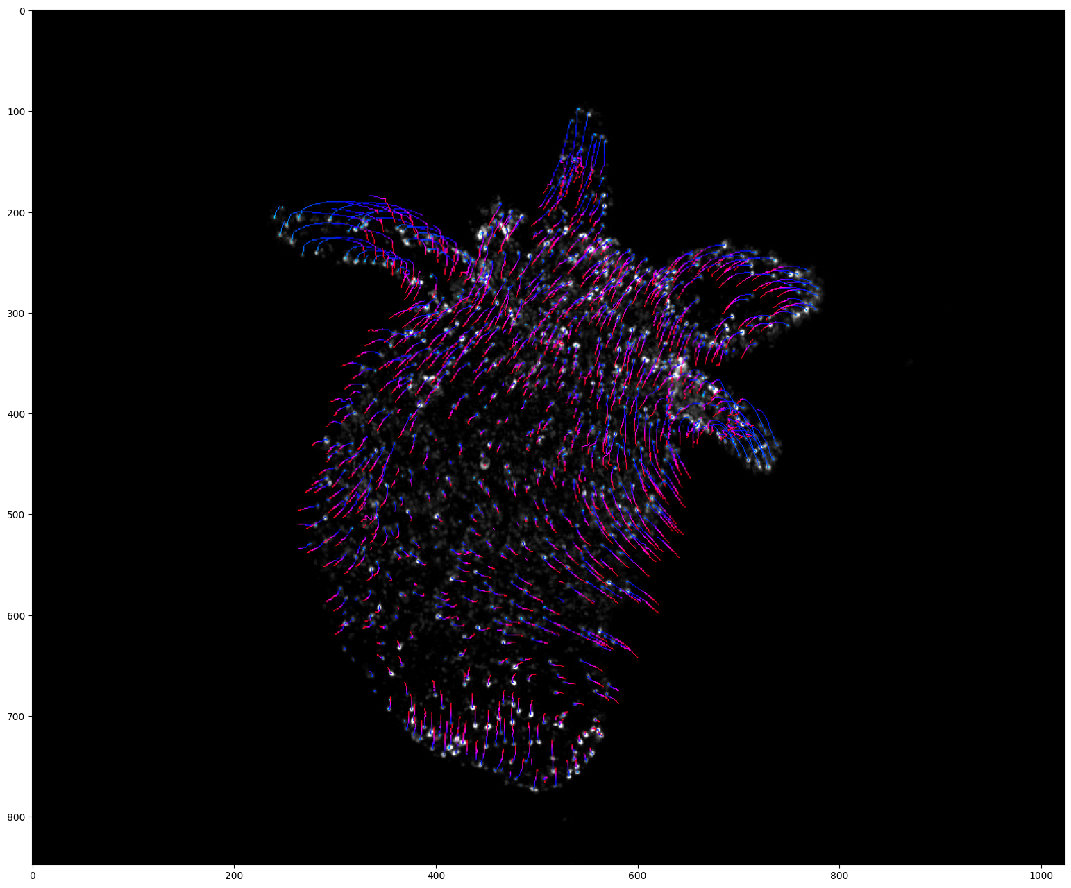
[25]:
# Project tracks onto a single image and color by time  (Only works with 2D videos)

# Create a list of colors for each time frame
# From cyan (start of the video) to red (end of the video)

hsv = mpl.colormaps["hsv"]
colors = [
    tuple(int(c * 255) for c in hsv(0.5 + 0.5 * k / (len(detections_sequence) - 1))[:3])
    for k in range(len(detections_sequence))
]

visu = byotrack.visualize.temporal_projection(
    byotrack.Track.tensorize(tracks), colors=colors, background=video[0], color_by_time=True
)

plt.figure(figsize=(24, 16))
plt.imshow(visu)
plt.show()
End-to-end tracking - Online or Offline tracking
[26]:
from byotrack import BatchMultiStepTracker, MultiStepTracker # noqa: F401
[27]:
# Create a full tracking pipeline from detector, linker and refiners
# If you have a BatchDetector and a OnlineLinker (True for WaveletDetector and KOFTLinker)
# You may use BatchMultiStepTracker that will process online the video (never keeping all the segmentations in RAM)
# Otherwise, use MultiStepTracker (Run Detections, then linking)

tracker = BatchMultiStepTracker(detector, linker, (smoother, stitcher, interpolater))
# tracker = MultiStepTracker(detector, linker, (smoother, stitcher, interpolater))
[28]:
tracks = tracker.run(video)
Merging 1022 tracks into 964 resulting tracks
[29]:
# Visualize track lifetime

byotrack.visualize.display_lifetime(tracks)

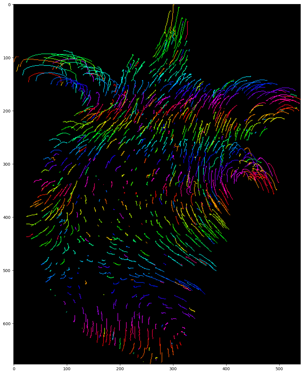
[30]:
# Project tracks onto a single image and color by track (Only works with 2D videos)

# Create a list of colors for each track (if more tracks than colors, it will cycle through it)

hsv = mpl.colormaps["hsv"]
colors = [tuple(int(c * 255) for c in hsv(k / 199)[:3]) for k in range(200)]

visu = byotrack.visualize.temporal_projection(
    byotrack.Track.tensorize(tracks),
    colors=colors,
)

plt.figure(figsize=(24, 16))
plt.imshow(visu)
plt.show()
[31]:
# Display the video, detections and tracks with Napari

viewer = byotrack.napari.visualize(video, detections_sequence, tracks)
Load or save tracks to files
[32]:
# Save tracks in ByoTrack format (compressed in a torch tensor)

byotrack.Track.save(tracks, "tracks.pt")

# Can be reload with
tracks = byotrack.Track.load("tracks.pt")
[33]:
# We also provide IO with Icy software

from byotrack import icy

icy.save_tracks(
    tracks, "tracks.xml"
)  # Note that holes should should be filled first with the ForwardBackwardInterpolater

# You can (re)load tracks from icy with
tracks = icy.load_tracks("tracks.xml")